One very important aspect of mining is deciding what material in a deposit is worth mining and processing, versus what material should be seen as waste. This decision is summarized by the cutoff grade policy. To understand what this is, we should first understand what the notion of ‘grade’ means, first. The grade of a chunk of rock is simply the amount of ‘good stuff’ (say, gold, copper or whatever...) that is in the rock. For example, you may find 1 gram of copper in a 100 gram chunk, and therefore conclude that the grade of the chunk is 1% copper by weight. The problem starts when, as a miner, you realize that you don’t actually know the grade of every cubic inch in the mineral deposit. After drilling you may have a notion of how rich the deposit is, but you never know what you’re going to get until it’s actually out of the ground and through the processing mill.
We say, therefore, that the grade of the deposit is a ‘spatial random variable’ - random, to represent the fact that you can’t be 100% successful in predicting what’s underground, and spatial, because every cubic inch can have a different grade.

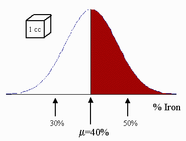
Now, the grade from every cubic inch can be thought of as a random draw from a statistical distribution. Iron deposits, for example, have grade distributions which are nearly normal. In the diagram, for example, the distribution of all 1 cc chunks in the deposit is normal with mean 40% Iron by weight, and standard deviation 10%. This means that out of 100 rocks, each one of size 1 cc, 50 are expected to have a grade greater than 40% Iron by weight (shown in red), and about 67 are expected to have a grade between 30% and 50% Iron by weight. This assumes that the rocks are picked far enough apart so that they are not related (in the words of statisticians, the samples are independent).
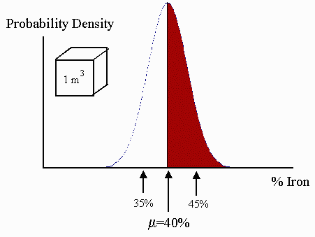
If, however, we consider chunks, much bigger than 1 cc in volume, then the grade distribution of the new, larger chunks will become narrower. To explain this without using heavy mathematics, consider a ‘large’ 1 m3 chunk. It is composed of lots of 1 cc pieces. The variation between the smaller 1 cc bits largely cancels out when we consider averaging over 106 of them. To restate, you will always get a larger variation when comparing individuals versus comparing groups. Thus the scattering of the larger blocks away from the mean will be smaller. This is shown in the next picture below.

Notice that the variation is smaller in the 1 m3 ‘block’ population, as compared to the 1 cc distribution...the standard deviation has shrunk to 5%.. Anyone who is familiar with the central limit theorem might ask, "why did the variation only decrease by a factor of two, when the larger block contains 106 of the smaller chunks?" Indeed, if all the 1 cc chunks were truly independent, the variation of the 1 m3 block distribution would be roughly 33 times smaller. The 1 cc chunks, however, are not independent from each other. One is more likely to find small variations between chunks close together than a mile apart. So, in turn, only this smaller amount of variation gets canceled when we average the grade of the 106 of chunks...precisely because they are situated close together and are not independent.
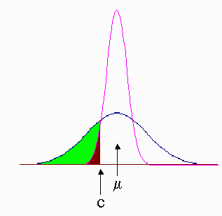
Now where does the cutoff grade decision enter all of this? Consider the following diagram:

The broad distribution corresponds to a small block distribution, say 1 cc chunks. The area underneath it (including the shaded bits) is 1.0
The narrower distribution corresponds to a large block distribution, say 1 m3, and the area underneath it (again, including the brown shaded part) is also 1.0 The mean grade of both distribution is the same, i.e. μ, and the cutoff grade has been specified to be c. Notice that the shaded parts of the two distributions are below the cutoff. We will throw that stuff out as waste. It’s easy to see that more of the broad (i.e. small block) distribution gets thrown out as waste. Thus, if we mine in larger blocks, we will throw out less and process more. The down side to this is that by throwing out less (i.e. not being as discriminate about what is allowed into the processing mill) we guarantee that the quality or grade of ore that is fed to the mill is poorer. Notice that this relationship ’flips’ if the cutoff is above the mean.
We can illustrate the above phenomenon with an example calculation based on the Iron ore distribution above. If we set the cutoff grade to be 30% Iron by weight, then the waste with 1 cc blocks is everything below one standard deviation left of the mean. From standard normal tables, this corresponds to 15.9% of the deposit. On the other hand, anyone mining with 1 m3 blocks would calculate that the cutoff grade is two standard deviations below the mean. This corresponds to 2.3% of the deposit being classified as waste...a large difference indeed. The mean of the material above the cutoff can be calculated using the formula

where σ is the standard deviation, P is the proportion of the deposit above the cutoff and Zc is the number of standard deviations between the cutoff and the mean grade, μ.
In the case of the 1 cc chunks, we use σ = 0.10, P = 0.841 and Zc = 1 to give μc = 42.9%.
In the case of 1 m3 blocks, we use σ = 0.05, P = 0.977 and Zc = 2 to give μc = 40.3%.
To summarize what we have learned:
- The grade distribution of a deposit must be specified along with a basic mining unit volume.
- For a given cutoff grade (below the mean), the smaller the basic mining block, the more material is thrown out as waste.
- For a given cutoff grade (below the mean), the smaller the basic mining block, the higher the mean grade of material above the cutoff grade.
This is known as the VOLUME-VARIANCE RELATIONSHIP