An Example of Using Maple™ to Solve Ordinary Differential Equations
1. Setting up the Equation
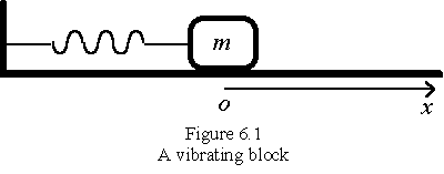
A metal block of mass, m=1.00 kg,
is attached to a spring having a stiffness k=4.00 N/m as
shown in Figure 6.1. When the block is displaced from the
equilibrium position o to a position
x, it will experience a restoring force that is
proportional to the displacement x and the spring
constant k. i. e.,
The negative sign means that the restoring force always points to the origin which is the equilibrium position of the block.
When the system vibrates in a medium such as water, oil, or air, the block will experience a resistance. In fact, all the vibrations die out in time because of the presence of damping forces. Provided the block moves slowly, the damping force is proportional to the block’s velocity:

where c is called the coefficient of viscous damping and the negative sign means that the damping force always points to the opposite direction of motion (velocity). In this example, we assume c= 1.00 N·s/m .
Therefore, according to Newton’s law of motion, F=ma , the motion of the vibrating block, in the presence of a viscous damping force, can be described by

This is a second-order ordinary differential equation. Here "order" refers to the highest order of derivative in the equation.
2. The General Solution
When we solve a differential equation, our goal is to find the unknown function, x(t), i.e., how x depends on t. Now let us use Maple™ to solve the differential equation (6.3).
First of all, we set up the differential equation in Maple™ and name it as "ode1":
>
  restart;
> ode1:=- k*x(t)-c*diff(x(t),t)=m*diff(x(t), t$2);

Caution:To indicate that x is a function of t, we have to use x(t) rather than simply x. Otherwise, Maple™ would treat x and t as two unrelated variables.
The command for solving
ordinary differential equations is
"dsolve":
> dsolve ({ode1},
  x(t));

This is a general solution for the vibrating block with damping. Since we have not used any initial conditions, the solution contains two arbitrary constants _C1 and _C2. In general, the solution of an nth order differential equation may have n arbitrary constants. When all the arbitrary constants are not determined, the solution is called a general solution. When at least one of these constants are determined, the solution is called a particular solution.
As we know, to determine the
arbitrary constants _C1 and _C2 in
x(t) we need two initial conditions, for example, the
initial displacement x(0) and the initial velocity x′(0). When we use Maple™, we can include the initial
conditions in the "dsolve"
command and find the particular solution.
dsolve({deqn, cond1,
  cond2}, x(t), option);
Please refer to the on-line help for details.
3. A ParticularSolution
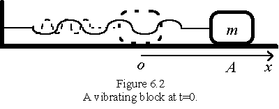
Now we pull the block to a
position ![]() metres from the equilibrium position as shown in
Figure 6.2 and then release it. If we define the time when we
release the block as
metres from the equilibrium position as shown in
Figure 6.2 and then release it. If we define the time when we
release the block as ![]() sec, find the displacement of the
block as a function of time.
sec, find the displacement of the
block as a function of time.
The differential equation is the same as that in example 6.1:
> restart;
> ode1:=-k*x(t)-c*diff(x(t),t)=m*diff(x(t), t$2);

The initial conditions are:
when t = 0,

> cond1:=x(0)=A;
cond1 := x(0) = A
> cond2:=D(x)(0)=0;
cond2 := D(x)(0) = 0
Attention:"D(x)(0)=0"
is the way (probably the only way) to represent x′(0) = 0 as an
initial condition. In Maple™, the Differential operator
"D" is used for representing
derivative functions. For example,
D(f)(a) is the derivative of the
function f at a, i.e., f′(a); while
(D@@3)(g)(b) would be the third
derivative of function g at b, i.e., g′′′(b).
> s62:=dsolve ({ode1, cond1,cond2}, x(t));

This is the particular solution that satisfies both the differential equation (6.3) and the initial conditions. Now let us substitute the specific values of m, k, c and A into the solution and plot it out:
> a62:=subs(m=1, k=4, c=1, A=2, s62):
> plot(rhs(a62), t=0..10);
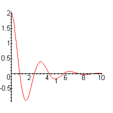
From the graph we can conclude that the metal block will vibrate with a decreasing amplitude and basically die out in about 10 seconds.
4. The "laplace" Option
The "dsolve" supports several options
such as the "laplace" option
and the "series" option, with
which sometimes we can obtain the solution in a more
understandable form. In fact, as shown below, with the
"laplace" option, the physical meanings of the solution
become more understandable.
> restart;
> ode1:=-k*x(t)-c*diff(x(t),t)=m*diff(x(t), t$2);

> cond1:=x(0)=A;
cond1 := x(0) = A
> cond2:=D(x)(0)=0;
cond2 := D(x)(0) = 0
> s64:=dsolve ({ode1, cond1, cond2}, x(t), laplace);
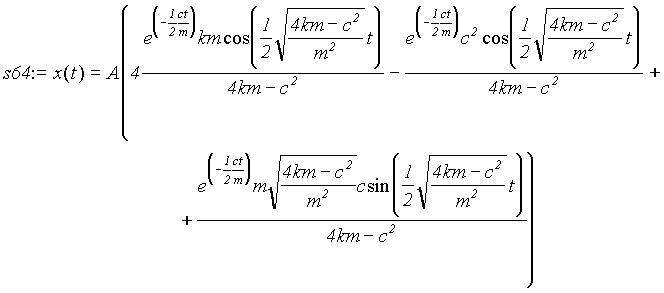
Each term in the solution is a sinusoidal function with an exponentially decaying amplitude, which exactly represents a dying-out vibration. Furthermore, it is straightforward to investigate how the parameters m, k, A and c affect the nature of the vibration.
5. The Damping Constant
For simplicity, we will substitute the value of the constants m, k, and A and investigate the meaning of the damping constant c by plotting the solution with different c values (c=1.00, 0.00, and 5.00).
> a64:=subs(m=1,k=4, A=2, s64);

> a641:=subs(c=1, a64);

> a640:=subs(c=0,a64);

> a645:=subs(c=5,a64);

> plot([rhs(a641), rhs(a640), rhs(a645)], t=0..10, thickness=[1,3,4]);
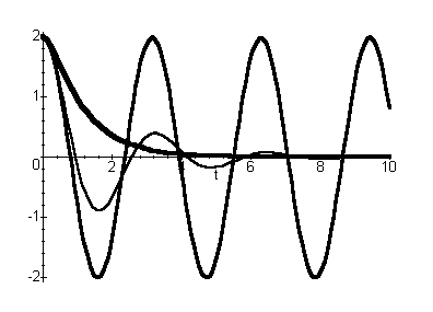
Also, we can use "plot3d" to have a complete
view of the displacement x as a function of time
t and the damping constant c:
> plot3d(rhs(a64), c=0..5, t=0..10);
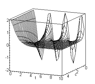
From the
two graphs above we can draw the following conclusions about the
damping constant c: When c = 0, there is no
damping, the block vibrates in a simple sinusoidal form, which is
call undamped vibration. When c=1, the block vibrates
with an exponentially decreasing amplitude, which is called
damped vibration or underdamped vibration. When c=5, the
block will not vibrate at all. Instead, it will approach the
equilibrium position obeying an exponential function, which is
called overdamped vibration. It is fairly straightforward to show
that the value of c to distinguish underdamped and
overdamped vibrations is given by ![]() which is called the value of
critical damping.
which is called the value of
critical damping.