BCIT ~ Mathematics

Background:

You are to design a new multi-channel temperature data logging system for use in the hospital in which you are working. The specifications given for its design are:

it is to be implemented around the Series 400 thermistor as a temperature probe,(such as YSI Series 400, or Thermometrics MA400)
it must provide temperature data to within 0.1°C from -40 to 100°C
it must have at least 6 independent channels each of which must be updated at least once every second
the data must be accessible to IBM/PC or compatible computers, via a standard RS-232 interface

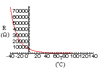
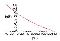
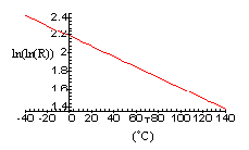
To convert the resistance, R, of the thermistors to a proportional voltage a constant current source is used. However, the problem that you immediately encounter is that the thermistors have an exponential response curve which makes direct digitization over the entire temperature range of interest difficult. You decide to linearize the voltage, as a function of temperature, prior to digitization by taking the double logarithm of the voltages measured across the thermistors, (the result of which is shown in Fig. 1).

Fig. 1: Plots of a) resistance, R, b) logarithm of the resistance, ln(R), and, c) double logarithm of the resistance, ln(ln(R)), as functions of temperature, T.

The process of taking the double logarithm of the analog signal is accomplished by the use of a pair of TL441AM logarithmic amplifiers (from Texas Instruments). The output voltage is then amplified and level shifted to give appropriate levels for the subsequent A/D converter. This being done, you collect the following data to see if your efforts have been justified:

Table 1: Thermistor Voltage and Temperature readings (after signal conditioning).

Temperature, T (°C)	-40	-20	0	20	40	60	80	100
Resistance, R (Ω)	75773.0	21862.1	7352.90	2813.11	1199.72	560.34	282.64	152.78
Output from log-amplifiers, (V)	4.579	3.970	3.369	2.775	2.185	1.594	0.999	0.399

The Problem

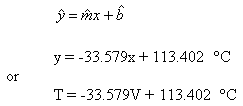
Find the equation of the best fit line (temperature as a function of voltage).
Determine 95% confidence intervals for the slope and y-int.
By looking at the results of (b) does it appear that the simple linear relation found in (a) is adequate to meet the specification of accuracy to within 0.1°C?

Solution

a) First find some intermediate results, (letting temperature be represented by 'y' and voltage by 'x').

Now using these results one can determine estimates for the slope, m, and the y-intercept, b.

yielding the following equation for the best fit line,

b) First determine some further intermediate results,

SSE = Syy - Sxy2/Sxx ≅16800-(-500.3)2/14.8990775 ≅ 0.2961257

where n=8, is the number of data points, and

t α/2, ν = t 0.025, 6 ≅ 2.447 (from table)

Now,

and,

c) As can be seen from the 95% CI for the y-intercept the simple linear relation found is not adequate to meet the specification of accuracy to within 0.1 ° C, (i.e. considering the y-int as an arbitrary predicted value, one cannot state with a reasonable degree of confidence, say 95% in this case, that the maximum error is less than ±0.4 °C).

FINAL NOTE:

The actual final design of the project discussed in this question was implemented using a single logarithmic amplifier to partially linearize the data (see Fig.1b) and a cubic spline curve fit to account for the remaining non-linearity. This approach not only met but exceeded the design specifications by providing temperature data to within 0.05 °C from -40 to 150 °C using a 12 bit plus sign serial I/O A/D converter. This method also allowed for simple calibration so as to account for the interchangeability tolerances of different probes. The reduced hardware and software associated with this method also allowed for increased speed making it possible to update each channel 60 times per second with real-time display via the RS-232 interface.

Electronics Statistics Example

Background:

The Problem

Solution

FINAL NOTE: